Predict Antimicrobial Resistance

Create a prediction model to predict antimicrobial resistance for the next years. Standard errors (SE) will be returned as columns se_min and se_max. See Examples for a real live example.

NOTE: These functions are deprecated and will be removed in a future version. Use the AMR package combined with the tidymodels framework instead, for which we have written a basic and short introduction on our website.

Usage

resistance_predict(x, col_ab, col_date = NULL, year_min = NULL,
  year_max = NULL, year_every = 1, minimum = 30, model = NULL,
  I_as_S = TRUE, preserve_measurements = TRUE, info = interactive(), ...)

sir_predict(x, col_ab, col_date = NULL, year_min = NULL, year_max = NULL,
  year_every = 1, minimum = 30, model = NULL, I_as_S = TRUE,
  preserve_measurements = TRUE, info = interactive(), ...)

# S3 method for class 'resistance_predict'
plot(x, main = paste("Resistance Prediction of",
  x_name), ...)

ggplot_sir_predict(x, main = paste("Resistance Prediction of", x_name),
  ribbon = TRUE, ...)

# S3 method for class 'resistance_predict'
autoplot(object,
  main = paste("Resistance Prediction of", x_name), ribbon = TRUE, ...)

Arguments

x: A data.frame containing isolates. Can be left blank for automatic determination, see Examples.
col_ab: Column name of x containing antimicrobial interpretations ("R", "I" and "S").
col_date: Column name of the date, will be used to calculate years if this column doesn't consist of years already - the default is the first column of with a date class.
year_min: Lowest year to use in the prediction model, dafaults to the lowest year in col_date.
year_max: Highest year to use in the prediction model - the default is 10 years after today.
year_every: Unit of sequence between lowest year found in the data and year_max.
minimum: Minimal amount of available isolates per year to include. Years containing less observations will be estimated by the model.
model: The statistical model of choice. This could be a generalised linear regression model with binomial distribution (i.e. using glm(..., family = binomial), assuming that a period of zero resistance was followed by a period of increasing resistance leading slowly to more and more resistance. See Details for all valid options.
I_as_S: A logical to indicate whether values "I" should be treated as "S" (will otherwise be treated as "R"). The default, TRUE, follows the redefinition by EUCAST about the interpretation of I (increased exposure) in 2019, see section Interpretation of S, I and R below.
preserve_measurements: A logical to indicate whether predictions of years that are actually available in the data should be overwritten by the original data. The standard errors of those years will be NA.
info: A logical to indicate whether textual analysis should be printed with the name and summary() of the statistical model.
...: Arguments passed on to functions.
main: Title of the plot.
ribbon: A logical to indicate whether a ribbon should be shown (default) or error bars.
object: Model data to be plotted.

Value

A data.frame with extra class resistance_predict with columns:

year
value, the same as estimated when preserve_measurements = FALSE, and a combination of observed and estimated otherwise
se_min, the lower bound of the standard error with a minimum of 0 (so the standard error will never go below 0%)
se_max the upper bound of the standard error with a maximum of 1 (so the standard error will never go above 100%)
observations, the total number of available observations in that year, i.e. $S + I + R$
observed, the original observed resistant percentages
estimated, the estimated resistant percentages, calculated by the model

Furthermore, the model itself is available as an attribute: attributes(x)$model, see Examples.

Details

Valid options for the statistical model (argument model) are:

"binomial" or "binom" or "logit": a generalised linear regression model with binomial distribution
"loglin" or "poisson": a generalised log-linear regression model with poisson distribution
"lin" or "linear": a linear regression model

Interpretation of SIR

In 2019, the European Committee on Antimicrobial Susceptibility Testing (EUCAST) has decided to change the definitions of susceptibility testing categories S, I, and R (https://www.eucast.org/newsiandr).

This AMR package follows insight; use susceptibility() (equal to proportion_SI()) to determine antimicrobial susceptibility and count_susceptible() (equal to count_SI()) to count susceptible isolates.

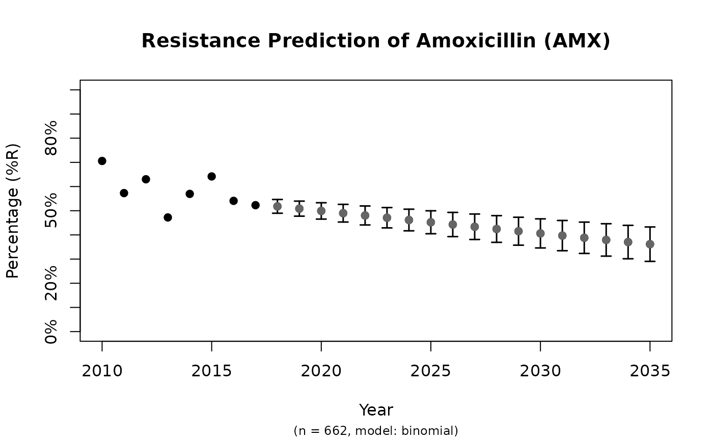
Examples

x <- resistance_predict(example_isolates,
  col_ab = "AMX",
  year_min = 2010,
  model = "binomial"
)
#> Warning: The resistance_predict() function is deprecated and will be removed in a
#> future version, see ?AMR-deprecated. Use the tidymodels framework
#> instead, for which we have written a basic and short introduction on our
#> website: https://amr-for-r.org/articles/AMR_with_tidymodels.html
#> This warning will be shown once per session.
plot(x)

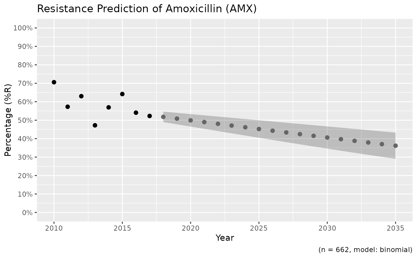
# \donttest{
if (require("ggplot2")) {
  ggplot_sir_predict(x)
}


# using dplyr:
if (require("dplyr")) {
  x <- example_isolates %>%
    filter_first_isolate() %>%
    filter(mo_genus(mo) == "Staphylococcus") %>%
    resistance_predict("PEN", model = "binomial")
  print(plot(x))

  # get the model from the object
  mymodel <- attributes(x)$model
  summary(mymodel)
}

#> NULL
#> 
#> Call:
#> glm(formula = df_matrix ~ year, family = binomial)
#> 
#> Coefficients:
#>             Estimate Std. Error z value Pr(>|z|)
#> (Intercept) 35.76101   72.29172   0.495    0.621
#> year        -0.01720    0.03603  -0.477    0.633
#> 
#> (Dispersion parameter for binomial family taken to be 1)
#> 
#>     Null deviance: 5.3681  on 11  degrees of freedom
#> Residual deviance: 5.1408  on 10  degrees of freedom
#> AIC: 50.271
#> 
#> Number of Fisher Scoring iterations: 4
#> 

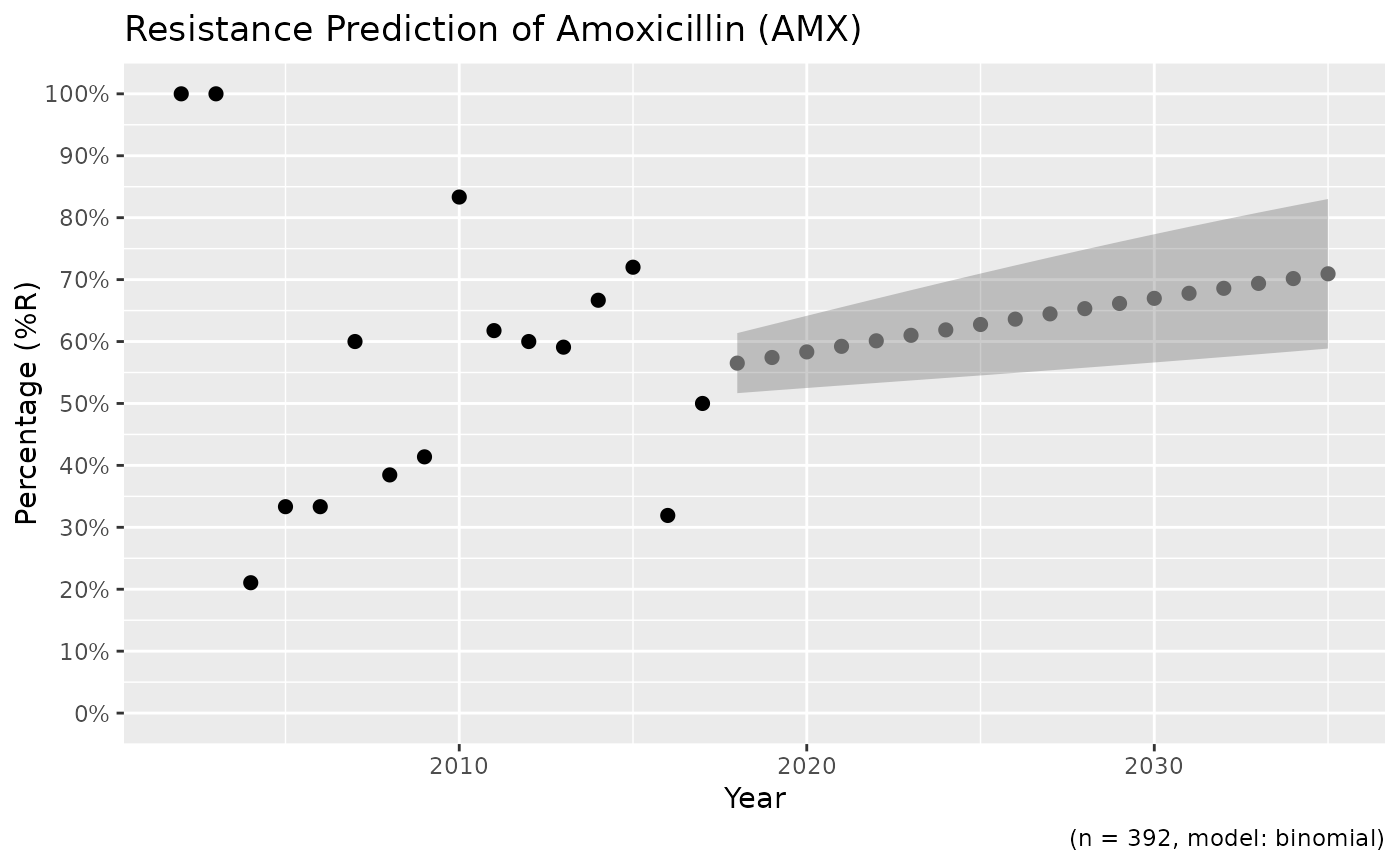
# create nice plots with ggplot2 yourself
if (require("dplyr") && require("ggplot2")) {
  data <- example_isolates %>%
    filter(mo == as.mo("E. coli")) %>%
    resistance_predict(
      col_ab = "AMX",
      col_date = "date",
      model = "binomial",
      info = FALSE,
      minimum = 15
    )
  head(data)
  autoplot(data)
}

# }