AMR Plots with ggplot2 — ggplot

Use these functions to create bar plots for AMR data analysis. All functions rely on ggplot2 functions.

Usage

ggplot_sir(
  data,
  position = NULL,
  x = "antibiotic",
  fill = "interpretation",
  facet = NULL,
  breaks = seq(0, 1, 0.1),
  limits = NULL,
  translate_ab = "name",
  combine_SI,
  minimum = 30,
  language = get_AMR_locale(),
  guideline = getOption("AMR_guideline", "EUCAST"),
  nrow = NULL,
  colours = c(S = "#3CAEA3", SDD = "#8FD6C4", SI = "#3CAEA3", I = "#F6D55C", IR =
    "#ED553B", R = "#ED553B"),
  datalabels = TRUE,
  datalabels.size = 2.5,
  datalabels.colour = "grey15",
  title = NULL,
  subtitle = NULL,
  caption = NULL,
  x.title = "Antimicrobial",
  y.title = "Proportion",
  ...
)

geom_sir(
  position = NULL,
  x = c("antibiotic", "interpretation"),
  fill = "interpretation",
  translate_ab = "name",
  minimum = 30,
  language = get_AMR_locale(),
  combine_SI,
  guideline = getOption("AMR_guideline", "EUCAST"),
  ...
)

labels_sir_count(
  position = NULL,
  x = "antibiotic",
  translate_ab = "name",
  minimum = 30,
  language = get_AMR_locale(),
  combine_SI,
  guideline = getOption("AMR_guideline", "EUCAST"),
  datalabels.size = 3,
  datalabels.colour = "grey15"
)

Arguments

data: A data.frame with column(s) of class sir (see as.sir()).
position: Position adjustment of bars, either "fill", "stack" or "dodge".
x: Variable to show on x axis, either "antibiotic" (default) or "interpretation" or a grouping variable.
fill: Variable to categorise using the plots legend, either "antibiotic" (default) or "interpretation" or a grouping variable.
facet: Variable to split plots by, either "interpretation" (default) or "antibiotic" or a grouping variable.
breaks: A numeric vector of positions.
limits: A numeric vector of length two providing limits of the scale, use NA to refer to the existing minimum or maximum.
translate_ab: A column name of the antimicrobials data set to translate the antibiotic abbreviations to, using ab_property().
combine_SI: (deprecated in favour of guideline) A logical. If set, it takes precedence over guideline: TRUE merges S, SDD, and I into "SI" vs. "R", and FALSE keeps S, I, and R separate.
minimum: The minimum allowed number of available (tested) isolates. Any isolate count lower than minimum will return NA with a warning. The default number of 30 isolates is advised by the Clinical and Laboratory Standards Institute (CLSI) as best practice, see Source.
language: Language of the returned text - the default is the current system language (see get_AMR_locale()) and can also be set with the package option AMR_locale. Use language = NULL or language = "" to prevent translation.
guideline: A guideline name, "EUCAST" or "CLSI" (or any version thereof, e.g. "CLSI 2025"), to determine whether the 'I' category is considered susceptible (EUCAST) or resistant (CLSI). The default is the package option AMR_guideline, or "EUCAST" if it is not set. For functions that return results per category, i.e., count_df(), proportion_df(), sir_df(), ggplot_sir(), geom_sir(), and labels_sir_count(), this can also be NULL or FALSE to keep S, I, and R separate. See section Interpretation of SIR below.
nrow: (when using facet) number of rows.
colours: A named vactor with colour to be used for filling. The default colours are colour-blind friendly.
datalabels: Show datalabels using labels_sir_count().
datalabels.size: Size of the datalabels.
datalabels.colour: Colour of the datalabels.
title: Text to show as title of the plot.
subtitle: Text to show as subtitle of the plot.
caption: Text to show as caption of the plot.
x.title: Text to show as x axis description.
y.title: Text to show as y axis description.
...: Other arguments passed on to geom_sir() or, in case of scale_sir_colours(), named values to set colours. The default colours are colour-blind friendly, while maintaining the convention that e.g. 'susceptible' should be green and 'resistant' should be red. See Examples.

Details

At default, the names of antimicrobials will be shown on the plots using ab_name(). This can be set with the translate_ab argument. See count_df().

geom_sir() will take any variable from the data that has an sir class (created with as.sir()) using sir_df() and will plot bars with the percentage S, I, and R. The default behaviour is to have the bars stacked and to have the different antimicrobials on the x axis.

Additional functions include:

facet_sir() creates 2d plots (at default based on S/I/R) using ggplot2::facet_wrap().
scale_y_percent() transforms the y axis to a 0 to 100% range using ggplot2::scale_y_continuous().
scale_sir_colours() sets colours to the bars (green for S, yellow for I, and red for R). with multilingual support. The default colours are colour-blind friendly, while maintaining the convention that e.g. 'susceptible' should be green and 'resistant' should be red.
theme_sir() is a ggplot2 theme with minimal distraction.
labels_sir_count() print datalabels on the bars with percentage and amount of isolates using ggplot2::geom_text().

ggplot_sir() is a wrapper around all above functions that uses data as first input. This makes it possible to use this function after a pipe (%>%). See Examples.

Interpretation of SIR

In 2019, the European Committee on Antimicrobial Susceptibility Testing (EUCAST) has decided to change the definitions of susceptibility testing categories S, I, and R (https://www.eucast.org/bacteria/clinical-breakpoints-and-interpretation/definition-of-s-i-and-r/).

In aggregated analyses, such as proportions, counts, antibiograms, and plots, the 'I' category must be considered either susceptible or resistant. In epidemiological AMR data analysis, this follows the guideline: EUCAST considers 'I' susceptible, while CLSI considers 'I' resistant. The dose-dependent susceptibility of CLSI ('SDD') is always considered susceptible, as it equals what EUCAST defines as 'I'. All functions with a guideline argument for this purpose use these categories:

`guideline`	Susceptible	Resistant
`"EUCAST"`	S, SDD, I, WT	R, NWT, NS
`"CLSI"`	S, SDD, WT	I, R, NWT, NS

The values 'WT' (wild type) and 'NWT' (non-wild type) result from epidemiological cut-off values (ECOFFs) instead of clinical breakpoints. Since they are no clinical categories, 'WT' is always considered susceptible and 'NWT' always resistant, regardless of the guideline. The value 'NS' (non-susceptible) is always considered resistant, and 'NI' (non-interpretable) is always considered a missing result.

The guideline argument can be:

Left unset, to use the package option AMR_guideline, or "EUCAST" if this option is not set. In the latter case, a message is shown once per session (but not in R Markdown or Quarto documents); set the option to silence it.
"EUCAST", or any EUCAST version such as "EUCAST 2025", to consider 'I' susceptible, e.g., to return "SI" vs. "R" in proportion_df().
"CLSI", or any CLSI version such as "CLSI 2025", to consider 'I' resistant, e.g., to return "S" vs. "IR" in proportion_df().
NULL or FALSE, to keep S, I, and R separate. This is only possible in functions that return results per category: count_df(), proportion_df(), sir_df(), ggplot_sir(), geom_sir(), labels_sir_count(), and bug_drug_combinations(). Functions that return a single proportion or count, such as susceptibility(), count_resistant(), antibiogram(), wisca(), and format() on the result of bug_drug_combinations(), require 'I' to be considered either susceptible or resistant, and return an error.

Use susceptibility() and resistance() (or count_susceptible() and count_resistant()) to follow the guideline, or e.g. proportion_SI() and proportion_R() to be explicit regardless of the guideline.

The combine_SI argument of the functions that return results per category, antibiogram(), and wisca() is deprecated in favour of guideline. If set, it is followed literally and takes precedence over guideline.

Examples

# \donttest{
if (require("ggplot2") && require("dplyr")) {
  # get antimicrobial results for drugs against a UTI:
  ggplot(example_isolates %>% select(AMX, NIT, FOS, TMP, CIP)) +
    geom_sir()
}
#> ℹ `geom_sir()` assumes the EUCAST guideline and thus considers the 'I' category
#>   susceptible (S+SDD+I vs. R). Use `guideline = "CLSI"` for S+SDD vs. I+R, or
#>   `guideline = NULL` to keep S, I, and R separate. Set the `guideline`
#>   argument, or set the `AMR_guideline` option to change the default (see
#>   `?AMR-options`). This message is shown once per session.

if (require("ggplot2") && require("dplyr")) {
  # prettify the plot using some additional functions:
  df <- example_isolates %>% select(AMX, NIT, FOS, TMP, CIP)
  ggplot(df) +
    geom_sir() +
    scale_y_percent() +
    scale_sir_colours(aesthetics = "fill") +
    labels_sir_count() +
    theme_sir()
}
#> ℹ `labels_sir_count()` assumes the EUCAST guideline and thus considers the 'I'
#>   category susceptible (S+SDD+I vs. R). Use `guideline = "CLSI"` for S+SDD vs.
#>   I+R, or `guideline = NULL` to keep S, I, and R separate. Set the `guideline`
#>   argument, or set the `AMR_guideline` option to change the default (see
#>   `?AMR-options`). This message is shown once per session.

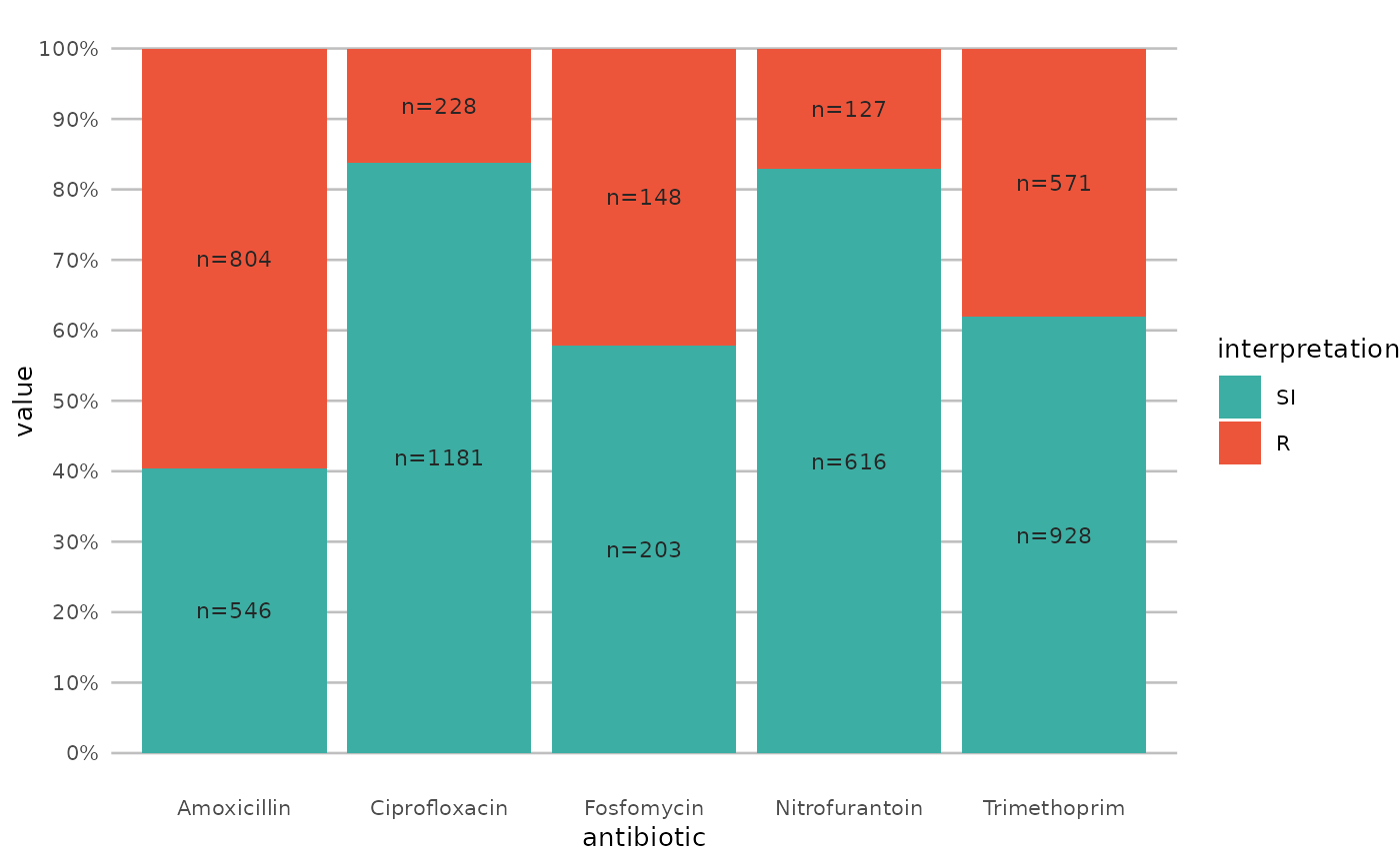if (require("ggplot2") && require("dplyr")) {
  # or better yet, simplify this using the wrapper function - a single command:
  example_isolates %>%
    select(AMX, NIT, FOS, TMP, CIP) %>%
    ggplot_sir()
}

if (require("ggplot2") && require("dplyr")) {
  # get only proportions and no counts:
  example_isolates %>%
    select(AMX, NIT, FOS, TMP, CIP) %>%
    ggplot_sir(datalabels = FALSE)
}

if (require("ggplot2") && require("dplyr")) {
  # add other ggplot2 arguments as you like:
  example_isolates %>%
    select(AMX, NIT, FOS, TMP, CIP) %>%
    ggplot_sir(
      width = 0.5,
      colour = "black",
      size = 1,
      linetype = 2,
      alpha = 0.25
    )
}
#> Warning: Ignoring unknown parameters: `size`

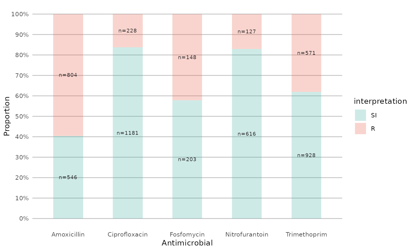if (require("ggplot2") && require("dplyr")) {
  # you can alter the colours with colour names:
  example_isolates %>%
    select(AMX) %>%
    ggplot_sir(colours = c(SI = "yellow"))
}

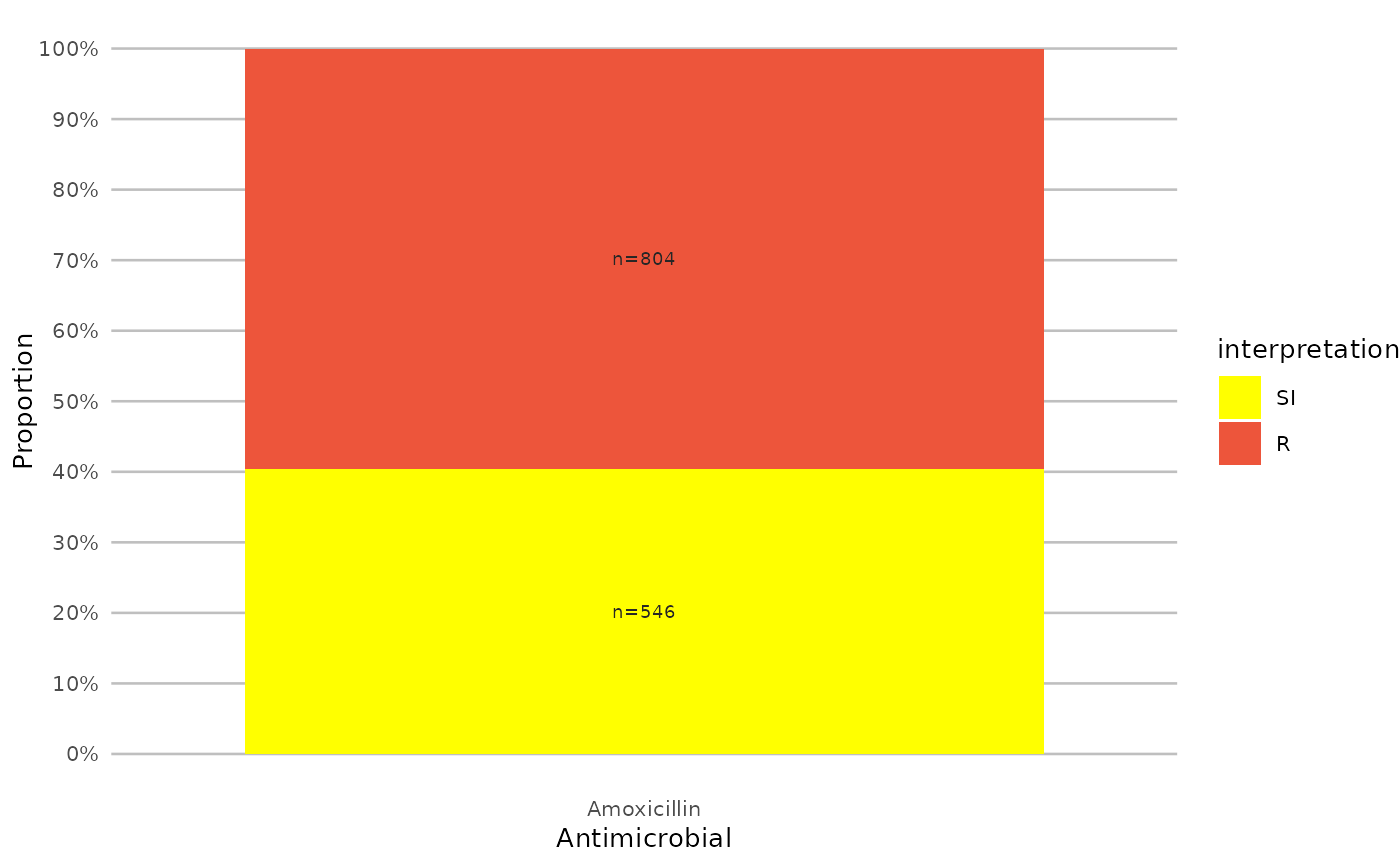if (require("ggplot2") && require("dplyr")) {
  # but you can also use the built-in colour-blind friendly colours for
  # your plots, where "S" is green, "I" is yellow and "R" is red:
  data.frame(
    x = c("Value1", "Value2", "Value3"),
    y = c(1, 2, 3),
    z = c("Value4", "Value5", "Value6")
  ) %>%
    ggplot() +
    geom_col(aes(x = x, y = y, fill = z)) +
    scale_sir_colours(
      aesthetics = "fill",
      Value4 = "S", Value5 = "I", Value6 = "R"
    )
}

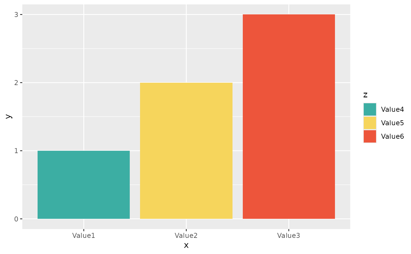if (require("ggplot2") && require("dplyr")) {
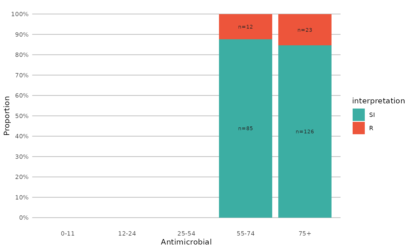
  # resistance of ciprofloxacine per age group
  example_isolates %>%
    mutate(first_isolate = first_isolate()) %>%
    filter(
      first_isolate == TRUE,
      mo == as.mo("Escherichia coli")
    ) %>%
    # age_groups() is also a function in this AMR package:
    group_by(age_group = age_groups(age)) %>%
    select(age_group, CIP) %>%
    ggplot_sir(x = "age_group")
}
#> Warning: Removed 6 rows containing missing values or values outside the scale range
#> (`geom_col()`).
#> Warning: Removed 6 rows containing missing values or values outside the scale range
#> (`geom_text()`).

if (require("ggplot2") && require("dplyr")) {
  # a shorter version which also adjusts data label colours:
  example_isolates %>%
    select(AMX, NIT, FOS, TMP, CIP) %>%
    ggplot_sir(colours = FALSE)
}

if (require("ggplot2") && require("dplyr")) {
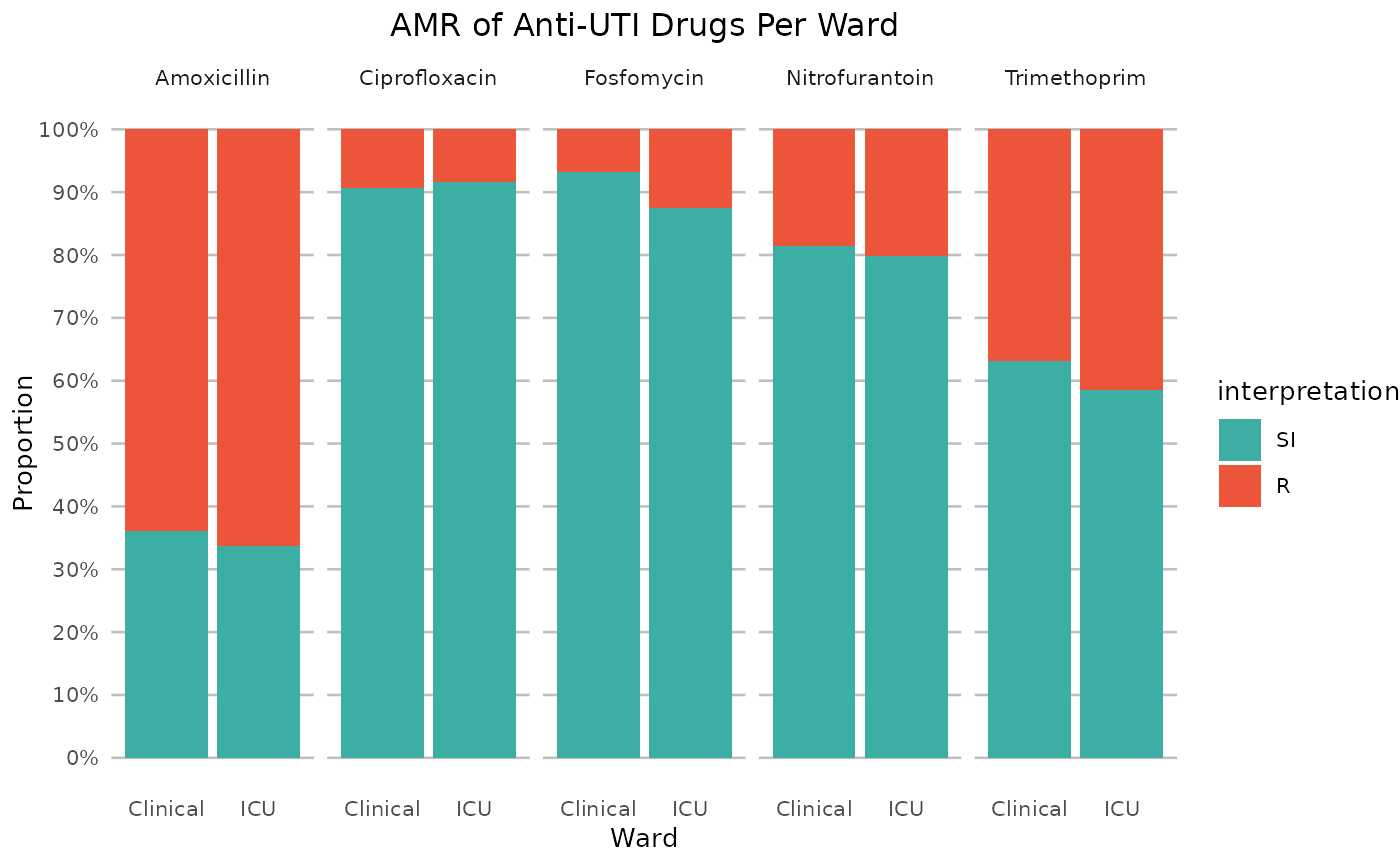
  # it also supports groups (don't forget to use the group var on `x` or `facet`):
  example_isolates %>%
    filter(mo_is_gram_negative(), ward != "Outpatient") %>%
    # select only UTI-specific drugs
    select(ward, AMX, NIT, FOS, TMP, CIP) %>%
    group_by(ward) %>%
    ggplot_sir(
      x = "ward",
      facet = "antibiotic",
      nrow = 1,
      title = "AMR of Anti-UTI Drugs Per Ward",
      x.title = "Ward",
      datalabels = FALSE
    )
}
#> ℹ Using column mo as input for `mo_is_gram_negative()`

# }